On movies

My favorites

I could just list the movies I have rated 10/10 over the years, but that would be not only underwhelming, it might also come across as a bit boring and predictable. Why? Well, because unsurprisingly, many of my all-time favorites are widely celebrated and universally recognized masterpieces. And really, isn’t that the point?

Naturally, I am talking about the Lord of the Rings trilogy, The Matrix, The Godfather I & II, Lawrence of Arabia, The Shawshank Redemption, and films by legends like Kubrick, Kurosawa, Hitchcock, Sergio Leone, and so on.

Instead, allow me to share five outstanding films, plus a few honorable mentions, that, while perhaps relatively well-known and having received a fair amount of attention, I believe not everyone has had the chance to watch or, in some cases, even hear of. Just to be clear, these suggestions reflect what came to mind on the particular day I wrote this. On another day, I might have come up with a completely different list. Let’s just say these are the ones that, with a bit of effort in digging through my memory, happened to rise to the surface.

Go watch them!

Just stating the obvious here: I am sure there are hundreds of excellent movies I have not seen yet. Hopefully, I will get the chance to watch them someday. In the meantime, I will keep doing my best and stay open to any recommendations.

12 Monkeys (1995)

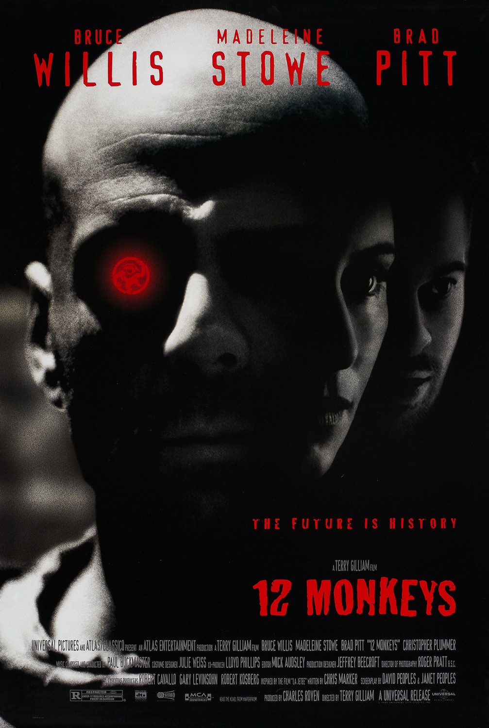
12 Monkeys is directed by Terry Gilliam, best known for his work with Monty Python. It’s an adaptation of the 1962 French short film La Jetée (directed by Chris Marker), a haunting piece composed entirely of still photographs (check it on YouTube).

Whenever I’m asked about my favorite time-travel movie, 12 Monkeys is always my answer. Gilliam is a master at making us feel the paranoia that consumes his characters. His framing and visual style often evoke discomfort and disorientation. Don’t believe me? Also watch Brazil, another one of his sublime works.

What makes 12 Monkeys so compelling to me, and why I have watched it countless times, is how it strips time-travel of its usual glamor and hopefulness. Instead, it presents a bleak, chaotic reality where time travel feels more like a punishment: ugly, confusing, and deeply unsettling. Brad Pitt gets most of the spotlight for his Oscar-nominated performance as a manic lunatic, but it is Bruce Willis who, in my opinion, truly carries the emotional weight. His portrayal of a man burdened by the impossible task of correcting the past is what sold me on the film’s tragic brilliance.

Honorable mentions in time-travel cinema: Primer (2004), Timecrimes (2007), Triangle (2009).

A Separation (2011)

I remember the first time I watched this film it felt like I was witnessing a documentary unfold. Nothing about it seems scripted, rehearsed, or even planned, and I mean that in the most positive way. It plays out as if a hidden camera were quietly capturing the steps, misfortunes, and emotional struggles of an ordinary family in Iran, desperately trying (or not?) to find balance within their household. The opening scene alone is enough to draw us in, highlighting the complexity and moral ambiguity behind the difficult choices people often face. Make no mistake: you won’t find happiness here. A Separation is an incredibly heartbreaking film, but one that absolutely deserves to be seen, rich in dialogue and emotional depth. I believe there is something profoundly human to be learned from it…

Honorable mentions in (dysfunctional) family drama: La graine et le mulet (2007), Kramer vs. Kramer (1979), Le Passé (2013), The Squid and the Whale (2005), Force Majeure (2014).

The Secret in Their Eyes (2009)

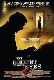
This Argentine-Spanish production won the Oscar for Best Foreign Language Film, so it’s hardly an obscure title that flew under the radar. Still, I believe it deserves a place on this list.

Technically impressive at times, its emotional impact lingers long after the credits roll. As I tried to process the implications of the choices made by certain characters, I found myself in one of those quiet, reflective moments, wondering: what would I have done?

Honorable mentions in films that might stir existential dread: Oldboy (2003), Contratiempo (2016), The Game (1997), Memento (2000), Ad Astra (2019), Aniara (2018).

Let the Bullets Fly (2010)

When it comes to Chinese comedies, much of the world tends to highlight the early works of Jackie Chan and, of course, Stephen Chow, whose Kung Fu Hustle and Shaolin Soccer are arguably the most universally acclaimed and widely recognized Chinese comedy films in the West. (Allow me to leave a big shoutout here to Zhang Yimou!)

However, overlooking Jiang Wen’s satirical masterpiece Let the Bullets Fly would be a mistake. As the title suggests, “letting the bullets fly” reflects a passive stance, that of hoping problems will resolve themselves without direct action. Unsurprisingly, this approach leads to questionable outcomes and raises serious moral dilemmas. Admittedly, having some familiarity with Chinese culture and society can deepen one’s appreciation of the film’s nuances and characters. But regardless of cultural background, this is a wildly chaotic and riotously funny movie that stands out in the genre.

Honorable mentions in Chinese cinema: Not One Less (1999), The Assassin (2015), A World without Thieves (2004), Blind Shaft (2003), Black Coal, Thin Ice (2014), Mr. Six (2015).

The Hunt (2012)

Ever wanted to watch a film that leaves you drowning in heartbreak and helpless rage? This is that movie. The kind that makes you want to scream at the screen, desperate to intervene.

It follows a kindergarten teacher caught in a devastating spiral of false accusations. Set in a seemingly idyllic village, the story unfolds in a place where the quiet charm of places and people, including friends, colleagues, and neighbors, masks a chilling refusal to hear the truth.

Forget the presumption of innocence. This is a harrowing tale of guilty until proven innocent. It is infuriating, gripping, and painfully relevant.

Honorable mentions in the fight for truth: The Lives of Others (2006), 12 Angry Men (1957), Prisoners (2014), Mystic River (2003), The Teachers’ Lounge (2023).

IMDb Data Analyzer

There was a time when IMDb provided user statistics within our profiles, but unfortunately, that’s no longer the case.

So, I’ve decided to code a basic (and far from perfect) Python script to bring those statistics back to life, along with some additional ones.

If you have any suggestions for the code or the types of statistics to include, please let me know.

You can check out the code here

To the best of my knowledge, GitHub Pages, Jekyll, and Jupyter Notebooks do not integrate seamlessly.

To display the notebook shown below, I used the Anaconda Prompt to generate a markdown file by running the following command:

jupyter nbconvert --to markdown < file name >.ipynb

Between this method and converting the notebook to HTML, I prefer the former.

Import libraries and load the CSV file with ratings.

You can obtain the ratings file from your IMDb user account.

import pandas as pd 
import numpy as np
import matplotlib.pyplot as plt
from datetime import date

ratings  =  pd.read_csv("ratings.csv")

print("Last updated:" + str(date.today()))

Last updated:2025-11-07

Parsing data.

Essentially, I will count the occurrences of each instance.

I am interested only in my own ratings, IMDb ratings, release year, and genres.

Please note that one movie can belong to multiple genres.

movie_idxs          = ratings.index[ratings['Title Type']=='Movie'].tolist()

my_movie_ratings    = ratings.iloc[movie_idxs,1]
counted_ratings     = np.unique(my_movie_ratings, return_counts=True)

imdb_ratings        = ratings.iloc[movie_idxs,7]

my_movie_years      = ratings.iloc[movie_idxs,9]
counted_years       = np.unique(my_movie_years, return_counts=True)

my_movie_runtimes   = ratings.iloc[movie_idxs,8]
counted_runtimes    = np.unique(my_movie_runtimes, return_counts=True)

my_movie_genres_aux = ratings.iloc[movie_idxs,10].str.split(", ") # the space after the comma is important
my_movie_genres     = [item for sublist in my_movie_genres_aux for item in sublist]
counted_genres      = np.unique(my_movie_genres, return_counts=True)

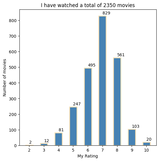
Plotting the distribution of my ratings.

The total number of movies I have given each score is indicated on top of each bar.

plt.figure(figsize=(6, 6), frameon=True)
plt.bar(counted_ratings[0], counted_ratings[1], color ='#4682B4', width = 0.5, edgecolor='wheat', linewidth=2)
 
plt.xlabel("My Rating")
plt.ylabel("Number of movies")
plt.xticks(counted_ratings[0])

for i in range(len(counted_ratings[0])):
    plt.text(counted_ratings[0][i], counted_ratings[1][i] + 10,
             str(counted_ratings[1][i]))

plt.title("I have watched a total of %d movies" %(sum(counted_ratings[1][:]))) 

plt.show()

Plotting information about the genres.

For better visualization, I will group less-watched genres into Others and limit the pie chart to eight wedges.

The popularity of each genre in the Others category is listed in the table below.

genres_dataframe = pd.DataFrame(
    data = {
        'Genre': counted_genres[0].tolist(),
        'value' : counted_genres[1].tolist()},
    ).sort_values('value', ascending = False)

# The top 7 most watched genres
genres_dataframe_most_watched = genres_dataframe[:7].copy()

# The remaining genres are summed up altogether
genres_dataframe_others = pd.DataFrame(data = {
    'Genre' : ['Others'],
    'value' : [genres_dataframe['value'][7:].sum()]
})

# Combine dataframes
genres_dataframe_compact = pd.concat([genres_dataframe_most_watched, genres_dataframe_others])

# I like blue :)
color_shades = ['#728FCE','#4863A0','#2B547E','#36454F', '#29465B','#2B3856','#123456', '#151B54']	

fig, ax = plt.subplots(figsize=(6, 6))

patches, texts, pcts = ax.pie(
    genres_dataframe_compact['value'], labels=genres_dataframe_compact['Genre'].tolist(), autopct='%.1f%%',
    colors=color_shades,
    wedgeprops={'linewidth': 2.0, 'edgecolor': 'wheat'},
    textprops={'size': 'large', 'fontweight': 'bold'})

# Set the corresponding text label color to the wedge's face color.
for i, patch in enumerate(patches):
    texts[i].set_color(patch.get_facecolor())

plt.setp(pcts, color='white')
plt.setp(texts, fontweight='bold')

ax.set_title('Most watched genres', fontsize=18)

plt.tight_layout()
plt.show()

genres_dataframe_less_watched = genres_dataframe[7:].copy()
genres_dataframe_less_watched.rename(columns = {'value':'Movies watched'}, inplace = True)
genres_dataframe_less_watched.style.set_table_styles(
    [
        {
            'selector': 'th',
            'props': [('background-color', '#D3D3D3')]
        },
    ]
)



print(genres_dataframe_less_watched.to_string(index=False))

      Genre  Movies watched
     Sci-Fi             417
    Romance             307
    Fantasy             290
     Horror             282
     Family             182
  Biography             134
  Animation             122
        War              85
    History              82
    Western              37
      Sport              36
Documentary              34
      Music              31
    Musical              29
  Film-Noir              15
  Talk-Show               1

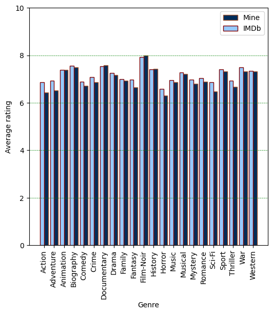
In the following, I will plot the average rate for each genre.

plt.figure(figsize=(6, 6))
 
plt.xlabel("Genre")
plt.ylabel("Average rating")

my_avg_genre_rating   = np.zeros([len(counted_genres[0])]) # Empty array
imdb_avg_genre_rating = np.zeros([len(counted_genres[0])]) # Empty array

for i, genre in enumerate(counted_genres[0]):
    for k in range(len(ratings['Genres'])):
        if (genre in str(ratings['Genres'][k])) and str(ratings['Title Type'][k]) == 'Movie':
            if genre == 'Music' and 'Musical' in str(ratings['Genres'][k]):
                # I am sure there's a better way to perform these loops :)
                pass
            else:
                my_avg_genre_rating[i] += ratings['Your Rating'][k]
                imdb_avg_genre_rating[i] += ratings['IMDb Rating'][k]

    my_avg_genre_rating[i] = my_avg_genre_rating[i]/counted_genres[1][i]
    imdb_avg_genre_rating[i] = imdb_avg_genre_rating[i]/counted_genres[1][i]

x_axis = np.arange(len(counted_genres[0]))
plt.bar(x_axis + 0.2, my_avg_genre_rating, width=0.4, label = 'Mine', color="#002c5a",edgecolor="sienna")
plt.bar(x_axis - 0.2, imdb_avg_genre_rating, width=0.4, label = 'IMDb', color="#96caff",edgecolor="maroon")
plt.xticks(x_axis,counted_genres[0])
plt.xticks(rotation=90)
plt.legend()
plt.grid(color = 'green', linestyle = '--', linewidth = 0.5)
plt.grid(axis = 'x')
plt.ylim([0, 10])
plt.show()

As somewhat expected for someone born in 1990, I have been watching more recent movies.

Additionally, only a few classics have stood the test of time.

plt.figure(figsize=(6, 6))
plt.bar(counted_years[0], counted_years[1], color ='#4682B4', width = 0.5, edgecolor="maroon",linewidth = 0.3)
 
plt.xlabel("Release year")
plt.ylabel("Number of movies")
plt.title("Release year of movies I've watched")

for i in range(0, len(counted_years[0]),5):
    plt.text(counted_years[0][i], counted_years[1][i] + 0.5,
             str(counted_years[1][i]),color='crimson',fontweight='bold')
plt.grid(color = 'blue', linestyle = '--', linewidth = 0.2)
plt.show()

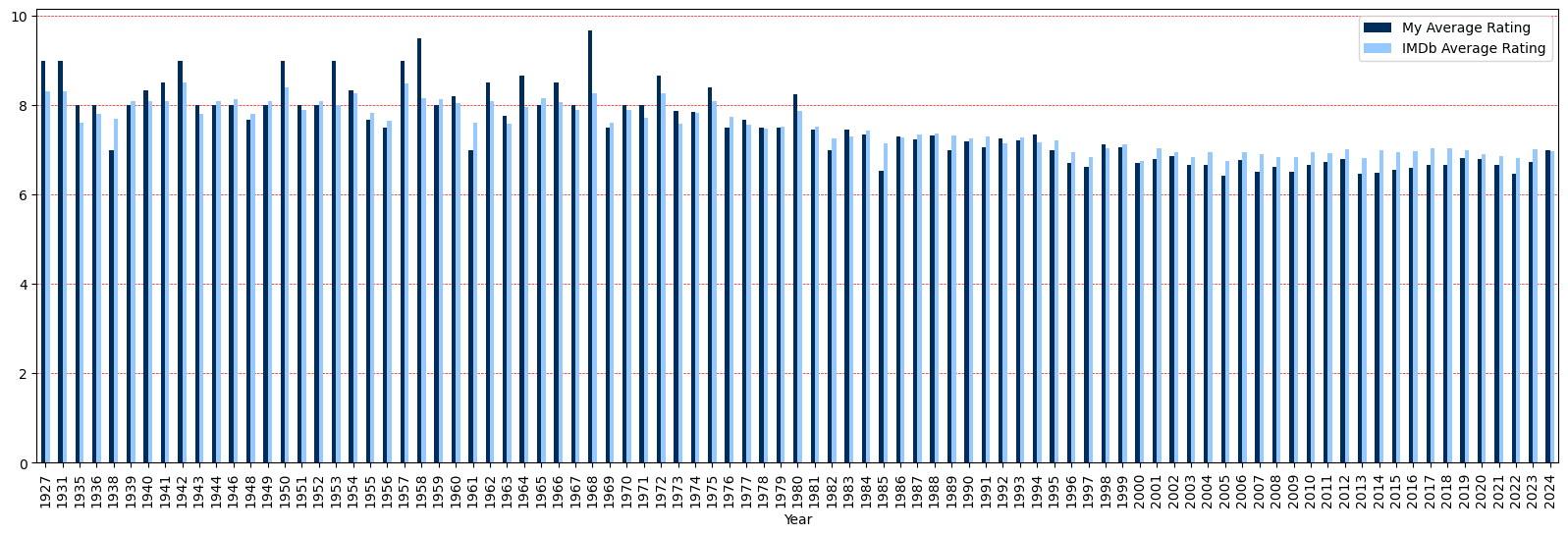
Let’s now take a look at the average ratings as a function of release year.

my_avg_rating   = np.empty([len(counted_years[0])]) # Empty array
imdb_avg_rating = np.empty([len(counted_years[0])]) # Empty array

for i in range(len(counted_years[0])):
    idxs = my_movie_years == counted_years[0][i]
    my_avg_rating[i]    = np.mean(my_movie_ratings[idxs])
    imdb_avg_rating[i]  = np.mean(imdb_ratings[idxs])

avg_ratings_df = pd.DataFrame({
    'Year': counted_years[0],
    'My Average Rating': my_avg_rating,
    'IMDb Average Rating': imdb_avg_rating
})

# plotting graph
ax = avg_ratings_df.plot(x="Year", y=["My Average Rating", "IMDb Average Rating"], kind="bar", figsize=(20, 6),
        subplots=False,
        grid=True,
        color={"My Average Rating": "#002c5a", "IMDb Average Rating": "#96caff"})
ax.set_axisbelow(True)
ax.grid(color='r', linestyle='--', linewidth=0.5)
ax.grid(axis='x')

Let’s now see how aligned I am with the masses.

It seems that we generally agree on the 7’s.

plt.figure(figsize=(6, 6))
plt.scatter(my_movie_ratings, imdb_ratings, alpha=0.5, edgecolors="k")
m, b = np.polyfit(my_movie_ratings, imdb_ratings, deg=1)

# Create a sequence of 50 points from 2 to 10 
sequence_x = np.linspace(counted_ratings[0][0], counted_ratings[0][-1], num=50)

# Plot regression line
plt.plot(sequence_x, b + m * sequence_x, color="dodgerblue", linestyle = '--', lw=1.5)

# Plot y = x line
plt.plot(sequence_x, sequence_x, color="darkgoldenrod", linestyle = '--', lw=1.5)

mean_rating = np.empty([len(counted_ratings[0])]) # Empty array
std_rating  = np.empty([len(counted_ratings[0])]) # Empty array

for i in range(len(counted_ratings[0])):
    idxs = my_movie_ratings == counted_ratings[0][i]
    imdb_ratings_aux = imdb_ratings[idxs]
    mean_rating[i] = np.mean(imdb_ratings_aux)
    std_rating[i] = np.std(imdb_ratings_aux)

plt.scatter(counted_ratings[0], mean_rating, color="crimson",edgecolors="orange")
plt.errorbar(counted_ratings[0], mean_rating, std_rating, fmt="o", color="r")
plt.xlabel('My rating')
plt.ylabel('IMDb rating')
plt.title('How much do I agree with IMDb ratings?')
plt.grid(color = 'blue', linestyle = '--', linewidth = 0.2)
plt.show()