 Macau, China
- University of Macau
- ResearchGate
- joelreis90
- Github
- Google Scholar
- ORCID
IMDb Data Analyzer
I love movies.
There was a time when IMDb provided some user statistics within our own profile. Not anymore…
I’ve decided to code a basic (and far from good) Python script to bring those and more statistics back to life.
If you have some suggestions for the code/statistics, please let me know.
You can check the code here
To the best of my knowledge, Github pages, Jekyll and Jupyter Notebooks do not play along very well.
In order to display the notebook seen below, I used the Anaconda Prompt to obtain a markdown file by running the following command:
jupyter nbconvert –to markdown < file name >.ipynb
Between this and converting the notebook to html, I prefer the former.
Import libraries and load csv file with ratings.
The ratings file is available from your IMDb user account.
import pandas as pd
import numpy as np
import matplotlib.pyplot as plt
from datetime import date

ratings  =  pd.read_csv("ratings.csv")

print("Last updated:" + str(date.today()))
Last updated:2024-01-10
Parsing data.
Basically, I shall count repetitions of an instance.
I am interested only in my own ratings, IMDb ratings, release year, and genres.
Note that one movie can have more than one genre.
movie_idxs          = ratings.index[ratings['Title Type']=='movie'].tolist()

my_movie_ratings    = ratings.iloc[movie_idxs,1]
counted_ratings     = np.unique(my_movie_ratings, return_counts=True)

imdb_ratings        = ratings.iloc[movie_idxs,6]

my_movie_years      = ratings.iloc[movie_idxs,8]
counted_years       = np.unique(my_movie_years, return_counts=True)

my_movie_runtimes   = ratings.iloc[movie_idxs,7]
counted_runtimes    = np.unique(my_movie_runtimes, return_counts=True)

my_movie_genres_aux = ratings.iloc[movie_idxs,9].str.split(", ") # the space after the comma is important
my_movie_genres     = [item for sublist in my_movie_genres_aux for item in sublist]
counted_genres      = np.unique(my_movie_genres, return_counts=True)
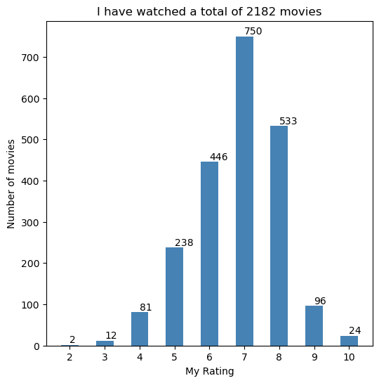
Plotting the distribution of my ratings.
On top of each bar I indicate the total number of movies which I have given that score.
plt.figure(figsize=(6, 6))
plt.bar(counted_ratings[0], counted_ratings[1], color ='#4682B4', width = 0.5)

plt.xlabel("My Rating")
plt.ylabel("Number of movies")
plt.xticks(counted_ratings[0])

for i in range(len(counted_ratings[0])):
    plt.text(counted_ratings[0][i], counted_ratings[1][i] + 5,
             str(counted_ratings[1][i]))

plt.title("I have watched a total of %d movies" %(sum(counted_ratings[1][:])))

plt.show()
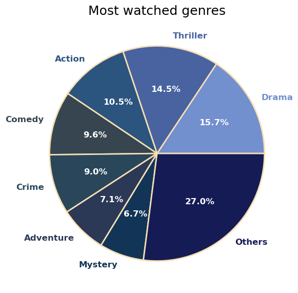
Plotting information about the genres.
For the sake of visualization, I will group less watched genres into Others and limit the pie chart to eight wedges.
The popularity of each of the Others genres is listed in the Table below.
genres_dataframe = pd.DataFrame(
    data = {
        'Genre': counted_genres[0].tolist(),
        'value' : counted_genres[1].tolist()},
    ).sort_values('value', ascending = False)

# The top 7 most watched genres
genres_dataframe_most_watched = genres_dataframe[:7].copy()

# The remaining genres are summed up altogether
genres_dataframe_others = pd.DataFrame(data = {
    'Genre' : ['Others'],
    'value' : [genres_dataframe['value'][7:].sum()]
})

# Combine dataframes
genres_dataframe_compact = pd.concat([genres_dataframe_most_watched, genres_dataframe_others])

# I like blue :)
color_shades = ['#728FCE','#4863A0','#2B547E','#36454F', '#29465B','#2B3856','#123456', '#151B54']

fig, ax = plt.subplots(figsize=(6, 6))

patches, texts, pcts = ax.pie(
    genres_dataframe_compact['value'], labels=genres_dataframe_compact['Genre'].tolist(), autopct='%.1f%%',
    colors=color_shades,
    wedgeprops={'linewidth': 3.0, 'edgecolor': 'white'},
    textprops={'size': 'x-large', 'fontweight': 'bold'})

# Set the corresponding text label color to the wedge's face color.
for i, patch in enumerate(patches):
    texts[i].set_color(patch.get_facecolor())

plt.setp(pcts, color='white')
plt.setp(texts, fontweight='bold')

ax.set_title('Most watched genres', fontsize=18)

plt.tight_layout()
plt.show()

genres_dataframe_less_watched = genres_dataframe[7:].copy()
genres_dataframe_less_watched.rename(columns = {'value':'Movies watched'}, inplace = True)
genres_dataframe_less_watched['#'] = [str(i + 8) for i in range(len(genres_dataframe_less_watched['Genre']))]
genres_dataframe_less_watched.set_index('#', inplace=True)
genres_dataframe_less_watched.style.set_table_styles(
    [
        {
            'selector': 'th',
            'props': [('background-color', '#D3D3D3')]
        },
        {
            'selector': 'tbody tr:nth-child(even)',
            'props': [('background-color', '#89CFF0')]
        }

    ]
)
| Genre | Movies watched | |
|---|---|---|
| # | ||
| 8 | Sci-Fi | 380 |
| 9 | Romance | 286 |
| 10 | Fantasy | 276 |
| 11 | Horror | 255 |
| 12 | Family | 179 |
| 13 | Biography | 129 |
| 14 | Animation | 116 |
| 15 | War | 84 |
| 16 | History | 73 |
| 17 | Western | 33 |
| 18 | Sport | 31 |
| 19 | Music | 29 |
| 20 | Musical | 28 |
| 21 | Documentary | 26 |
| 22 | Film-Noir | 15 |
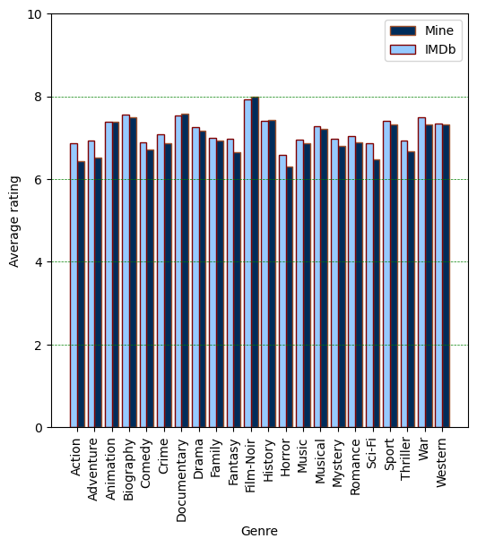
In the following, I will plot the average rate for each genre.
plt.figure(figsize=(6, 6))

plt.xlabel("Genre")
plt.ylabel("Average rating")

my_avg_genre_rating   = np.zeros([len(counted_genres[0])]) # Empty array
imdb_avg_genre_rating = np.zeros([len(counted_genres[0])]) # Empty array

for i, genre in enumerate(counted_genres[0]):
    for k in range(len(ratings['Genres'])):
        if (genre in str(ratings['Genres'][k])) and str(ratings['Title Type'][k]) == 'movie':
            if genre == 'Music' and 'Musical' in str(ratings['Genres'][k]):
                # I am sure there's a better way to perform these loops :)
                pass
            else:
                my_avg_genre_rating[i] += ratings['Your Rating'][k]
                imdb_avg_genre_rating[i] += ratings['IMDb Rating'][k]

    my_avg_genre_rating[i] = my_avg_genre_rating[i]/counted_genres[1][i]
    imdb_avg_genre_rating[i] = imdb_avg_genre_rating[i]/counted_genres[1][i]

x_axis = np.arange(len(counted_genres[0]))
plt.bar(x_axis + 0.2, my_avg_genre_rating, width=0.4, label = 'Mine')
plt.bar(x_axis - 0.2, imdb_avg_genre_rating, width=0.4, label = 'IMDb')
plt.xticks(x_axis,counted_genres[0])
plt.xticks(rotation=90)
plt.legend()
plt.grid(color = 'green', linestyle = '--', linewidth = 0.5)
plt.grid(axis = 'x')
plt.ylim([0, 10])
plt.show()
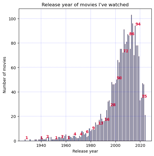
As somewhat expected for someone born in 1990, I have been watching more movies from recent times.
Moreover, only a few classics stand the test of time.
plt.figure(figsize=(6, 6))
plt.bar(counted_years[0], counted_years[1], color ='#4682B4', width = 0.5)

plt.xlabel("Release year")
plt.ylabel("Number of movies")
plt.title("Release year of movies I've watched")

for i in range(0, len(counted_years[0]),5):
    plt.text(counted_years[0][i], counted_years[1][i] + 0.5,
             str(counted_years[1][i]),color='red',fontweight='bold')
plt.grid(color = 'blue', linestyle = '--', linewidth = 0.2)
plt.show()
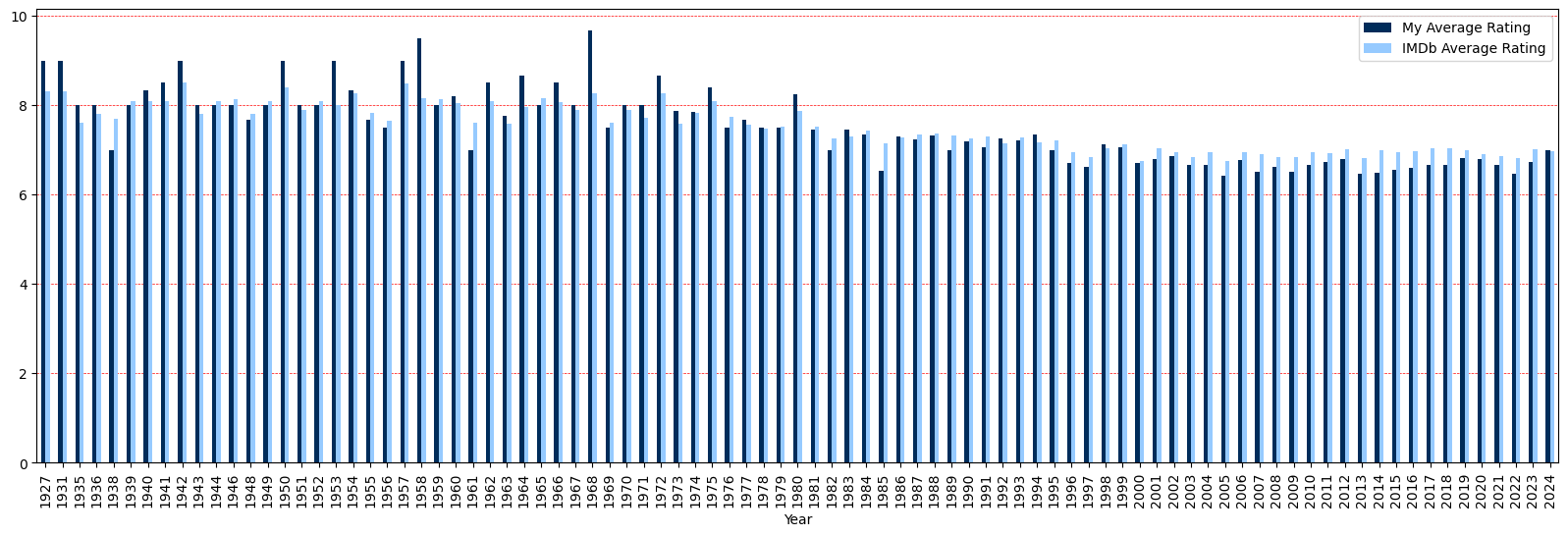
Let us now take a look at the average ratings in function of release year.
my_avg_rating   = np.empty([len(counted_years[0])]) # Empty array
imdb_avg_rating = np.empty([len(counted_years[0])]) # Empty array

for i in range(len(counted_years[0])):
    idxs = my_movie_years == counted_years[0][i]
    my_avg_rating[i]    = np.mean(my_movie_ratings[idxs])
    imdb_avg_rating[i]  = np.mean(imdb_ratings[idxs])

avg_ratings_df = pd.DataFrame({
    'Year': counted_years[0],
    'My Average Rating': my_avg_rating,
    'IMDb Average Rating': imdb_avg_rating
})

# plotting graph
ax = avg_ratings_df.plot(x="Year", y=["My Average Rating", "IMDb Average Rating"], kind="bar", figsize=(20, 6),
        subplots=False,
        grid=True,
        color={"My Average Rating": "#4682B4", "IMDb Average Rating": "#FFA500"})
ax.set_axisbelow(True)
ax.grid(color='r', linestyle='--', linewidth=0.5)
ax.grid(axis='x')
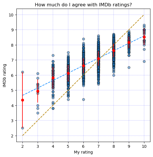
Let us see now how aligned I am with the masses.
It seems that we kind of agree on the 7’s.
plt.figure(figsize=(6, 6))
plt.scatter(my_movie_ratings, imdb_ratings, alpha=0.5, edgecolors="k")
m, b = np.polyfit(my_movie_ratings, imdb_ratings, deg=1)

# Create a sequence of 50 points from 2 to 10
sequence_x = np.linspace(counted_ratings[0][0], counted_ratings[0][-1], num=50)

# Plot regression line
plt.plot(sequence_x, b + m * sequence_x, color="r", linestyle = '--', lw=1.5)

# Plot y = x line
plt.plot(sequence_x, sequence_x, color="g", linestyle = '--', lw=1.5)

mean_rating = np.empty([len(counted_ratings[0])]) # Empty array
std_rating  = np.empty([len(counted_ratings[0])]) # Empty array

for i in range(len(counted_ratings[0])):
    idxs = my_movie_ratings == counted_ratings[0][i]
    imdb_ratings_aux = imdb_ratings[idxs]
    mean_rating[i] = np.mean(imdb_ratings_aux)
    std_rating[i] = np.std(imdb_ratings_aux)

plt.scatter(counted_ratings[0], mean_rating, color="r",edgecolors="orange")
plt.errorbar(counted_ratings[0], mean_rating, std_rating, fmt="o", color="r")
plt.xlabel('My rating')
plt.ylabel('IMDb rating')
plt.title('How much do I agree with IMDb?')
plt.grid(color = 'blue', linestyle = '--', linewidth = 0.2)
plt.show()